As diversified systematic trend followers, we just love the positive skew of our trade results….but to explain why, we need to dig quite deeply into what skewness means exactly.
It is defined as a measure of asymmetry of a trade distribution about its mean and is expressed by the following formula.

Now it is important to note that the formula above assumes that a particular distribution can be categorized as having a single mean and a single standard deviation around this mean, which is an inherently Gaussian assumption. We ‘as realists’ however understand that over large data samples, ‘real markets’ and ‘real trade results’ are more complex than that, and may frequently comprise multiple means and varying standard deviations that reflect different market conditions. However, despite this failing of the skewness formula when being applied to real distributions of complex adaptive systems such as these financial markets, we can simplify skewness to refer to the asymmetry between the magnitude of average wins and the average losses of the distribution of trade results.
Just don’t get too prescriptive in your use of these damned single measure statistics of theoretical distributions.
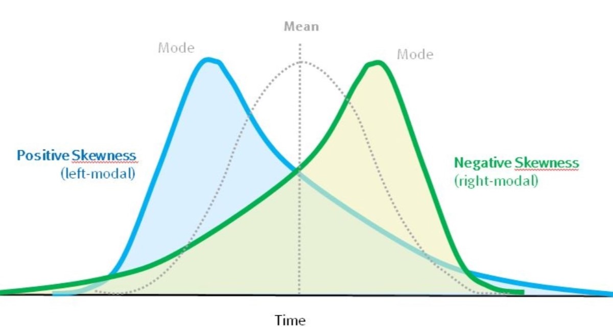
For example where our average winners are far greater than our average losers, our trade distribution histogram plots as a distribution with clear positive skew. If our average winners were far smaller than our average losers, then our trade distribution would plot with clear negative skew. The direction of the tails of these asymmetric distributions signify their ability to address the risk arising when real markets start to display exotic fat tailed behaviour.
What we mean is that the extremal value of a skewed distribution such as the maximum loss or the maximum win signifies where bias in the trade lies when exposed to the Power Laws found in ‘fat tailed’ environments. When conditions extend beyond the Gaussian envelope into the exotic tails of a distribution, events considered to be far less frequent actually become far more frequent than what a Normal distribution would imply. So for negative skewed systems, large losses are far more frequent than anticipated and for positive skewed systems, large wins are far more frequent than anticipated.
Chart 1 below reflects a trade distribution with positive skew. There is a long right tail to the distribution of trade results. While the vast proportion of trades are small losses, you can see that the exceptional winners result in the average win being far higher than the average loss. This feature creates a positive skew to the distribution of trade returns in this example.
Chart 1: Histogram of Trade Results of a Trend Following System with Positive Skew

The distribution of trade results in Chart 1 above applies to a trend following system comprising 237 trades undertaken between 1st January 2000 to today with an equity curve that is displayed in Chart 2 below.
Chart 2: Equity Curve of a Trend Following System comprising 237 trades

Now the reason that we like positive skew of our trade results is that under non-linear market conditions, the beneficial outlier can exponentially outweigh all the small losses associated with our trend following technique that cuts losses short at all times but lets profits run. This can be attributed to the Power Laws that reside in ‘Fat Tailed market environments. Trade events in the tails of the distribution can be many orders of magnitude greater than the trade events that lie within more ‘normal’ bounds of the trade distribution’.
Whether a system has positive or negative skew is important when considering the unforeseen risks associated with ‘fat tailed’ environments. A system with negative skew provides a ‘risk signature of weakness’ where the occasional large loss, under ‘fat tailed’ non-Gaussian market conditions can turn into exponentially larger losses than expected, particular when large losses become consecutive in nature.
Positively skewed systems on the other hand demonstrate through their risk signature that they are ‘robust’ and do not leave themselves open to the possibility of large losses. By always cutting losses short there is no exponential increase in losses when conditions become unfavorable as all adverse tail events are excluded from the trade history. There may be more small losses, but these events are not exponential in nature. Of course, by letting profits run, the trend follower leaves themselves open to the possibility of ‘exponential profits’ associated with favorable tail events.
Now that we understand the significance of skewness to non-linear risk events, lets now turn to the question of how we accurately measure skewness? As skewness is often incorrectly applied by the statistician.
How to Measure Skewness
The first point we need to understand when assessing the skewness arising from trend following systems is that we need to eliminate effects in the distribution that may arise from money management methods deployed by the system.
For example the trade results of the trend following system described in Charts 1 and 2 display compounded effects. In this system we applied a 1% trade risk of equity for each trade. This means that the trade results include the impacts of compounding in their signature. So we cannot use $ profit or $ loss per trade as a basis to calculate skew as these raw results will include effects of compounding. Rather we need to apply a method that normalises the trade results to exclude the impacts of money management method to ‘truly see’ the real skew in the system results.
So in the following examples we will be using a % of equity as a method to normalise the trade results. We could also apply an ATR or R multiple for each trade as well to achieve the same outcome.
The following table displays the skew of various methods applied to the trade results.

Now the question we need to ask when referring to the skew, is which result is ‘correct’?
Well we need to understand that all these different interpretations of skew arise from the same system result. The only difference is in how these results are consolidated.
The ‘correct’ result is actually represented by the ‘Trade Results’ column of 1.32. This skew calculation reflects the actual asymmetry of all trade results.
The Daily results and the Monthly Results column compound the skew by virtue of the fact that these methods consolidate trade results into a daily or monthly record. The consolidation process actually compounds the skew of positively skewed systems. The reason for this compounded nature through consolidation is that we are altering the skew of the distribution through consolidation. With classic trend following models outside periods of ‘Outlier’, most of our trades are losses. As we consolidate these losses the relative disparity between our Outliers and linear sequence of losses becomes more extreme leading to higher overall skew in the distribution. This effect compounds the asymmetry in the series.
We therefore need to be particularly careful in how we use skew to compare between alternatives. Ensure that you choose a particular method and stick with it. Unfortunately when assessing the skew between different Fund Managers based on available data, you sometimes only have monthly return data to work with and cannot determine the ‘real skew’ of the method….but it helps to be aware of these issues arising from the way we measure skew.
Anyway….enough of the rambling. Let’s hope you just don’t skew things up the next time you use it.
Trade well and prosper.